|
1
2
3
4
5
6
7
8
9
10
11
12
13
14
15
16
17
18
19
20
21
22
23
24
25
26
27
28
29
30
31
32
33
34
35
36
37
38
39
40
41
42
43
44
45
46
47
48
49
50
51
52
53
54
55
56
57
58
59
60
61
62
63
|
import numpy as np
import tensorflow as tf
import matplotlib.pyplot as plt
from tensorflow.keras.models import Sequential
from tensorflow.keras.layers import Flatten, Dense
from tensorflow.keras.optimizers import SGD, Adam
print(tf.__version__)
# 데이터셋 생성
x_data = np.random.randint(0, 11, size=(5, 3))-5 # -5~5
y_data = np.array([2*x[0] - x[0] + 3 * x[0] for x in x_data]) # y = 2x_1 - x_2 + 3x_3
print(x_data.shape, y_data.shape) # (5, 3) (5,)
# 모델 구축
model = Sequential()
model.add(Dense(10, input_shape=(3, ), activation='linear'))
model.add(Dense(1, activation='linear'))
# 모델 컴파일
model.compile(optimizer=SGD(learning_rate=1e-2), loss='mse')
model.summary()
# 모델 입출력 크기 확인
print(model.input)
print(model.output)
print(model.weights)
# 모델 학습
hist = model.fit(x_data, y_data, epochs=50)
# 모델 평가 및 예측
test_data = np.random.randint(0, 11, size=(5, 3))-5
test_data_label = np.array([2*x[0] - x[0] + 3 * x[0] for x in test_data])
pred_val = model.predict(test_data)
print(pred_val)
print(test_data_label)
# 모델 저장 및 로드
# model.save("model_name.h5")
# model = tf.keras.models.load_model("model_name.h5")
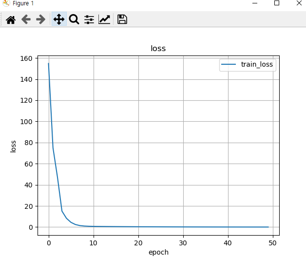
# 모델 손실함수 추이확인
plt.title("loss")
plt.xlabel("epoch")
plt.ylabel("loss")
plt.grid()
plt.plot(hist.history['loss'], label='train_loss')
plt.legend(loc='best')
plt.show()
|
cs |
위의 소스코드를 실행시키면 아래와 같은 출력값을 얻을 수 있다.

반응형
'머신러닝_딥러닝 > Tensorflow + Keras' 카테고리의 다른 글
| (Tensorflow 2.x) Logistic Regression 1탄 (0) | 2021.10.23 |
|---|---|
| (Tensorflow 2.x) Regression 2탄 (0) | 2021.10.23 |
| MNIST 2탄 (Back Propagation) (0) | 2021.10.23 |
| MNIST 1탄 (0) | 2021.10.23 |
| XOR 문제 (딥러닝으로 해결) (0) | 2021.10.23 |