|
1
2
3
4
5
6
7
8
9
10
11
12
13
14
15
16
17
18
19
20
21
22
23
24
25
26
27
28
29
30
31
32
33
34
35
36
37
38
39
40
41
42
43
44
45
46
47
48
49
50
51
52
53
54
55
56
57
58
59
60
61
62
63
64
65
66
67
68
69
70
71
72
73
74
75
76
77
78
79
80
81
82
|
import numpy as np
import tensorflow as tf
import matplotlib.pyplot as plt
from tensorflow.keras.datasets import imdb
from tensorflow.keras.models import Sequential
from tensorflow.keras.layers import Flatten, Dense
from tensorflow.keras.optimizers import SGD, Adam
print(tf.__version__)
# 데이터셋 생성
# imdb 데이터셋 => 영화 리뷰(이진 분류)
(x_train, y_train), (x_test, y_test) = imdb.load_data(num_words=10000) # 가장 자주 나타나는 단어 1만개만 사용
print(x_train.shape, y_train.shape)
print(x_train[0]) # data type = list, numpy(x), 리스트를 텐서로 바꿔줘야 함
print(y_train[0])
print(max([max(str) for str in x_train])) # 단어를 1만개로 제한 -> 단어 인덱스 최대 9,999
def vectorize(seq, dim=10000):
result = np.zeros((len(seq), dim))
for idx, val in enumerate(seq):
result[idx, val] = 1.
return result
x_train = vectorize(x_train) # (25000, 10000)
x_test = vectorize(x_test)
print(x_train[0])
y_train = np.asarray(y_train).astype("float32")
y_test = np.asarray(y_test).astype("float32")
# 데이터의 내용 확인방법
# w_index = imdb.get_word_index() # 단어를 정수 인덱스로 매핑한 딕셔너리
# rev_index = dict([(value, key) for (key, value) in w_index.items()]) # 단어와 정수 인덱스를 바꿈
# word_test = ' '.join([rev_index.get(i-3, '?') for i in x_train[0]]) # 원본 데이터의 3번째까지는 데이터 정보, '?'디폴트값
# print(word_test)
# 모델 구축
model = Sequential()
model.add(Dense(16, activation='relu', input_shape=(10000,)))
model.add(Dense(16, activation='relu'))
model.add(Dense(1, activation='sigmoid'))
# 모델 컴파일 (모델을 로드하는 부분에서 수행함)
model.compile(optimizer='rmsprop', loss='binary_crossentropy', metrics=['accuracy'])
# 모델 학습
history = model.fit(x_train, y_train, validation_split=0.4, epochs=20, batch_size=512)
print(history.history.keys()) # dict_keys(['loss', 'accuracy', 'val_loss', 'val_accuracy'])
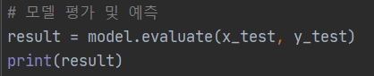
# 모델 평가 및 예측
# 모델 저장 및 로드
# model.save("model_name.h5")
# model = tf.keras.models.load_model("model_name.h5")
# 모델 손실함수 추이확인
loss = history.history['loss']
val_loss = history.history['val_loss']
epochs = range(1, len(loss)+1)
plt.plot(epochs, loss, 'bo', label="train_loss")
plt.plot(epochs, val_loss, 'b', label="val_loss")
plt.xlabel("epoch")
plt.ylabel("loss")
plt.legend(loc='best')
plt.show()
|
cs |
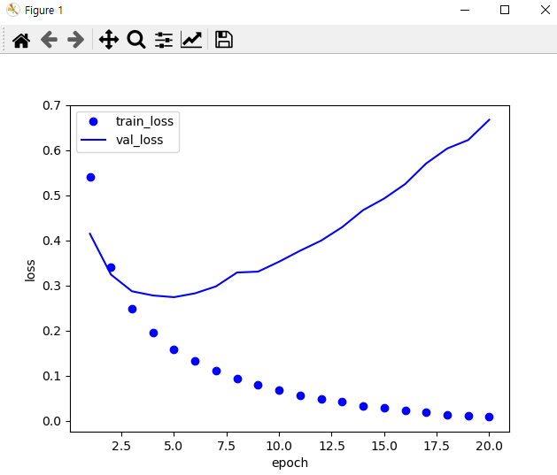
위의 소스코를 실행시키면 아래와 같은 출력값을 얻을 수 있다 -> 대략, epoch=5 가 적당하다.
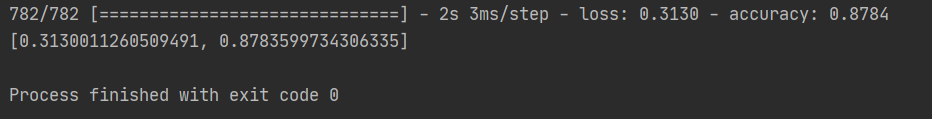
epoch=5로 하여 모델을 다시 학습시킨 후, 정확도를 확인해보면 아래와 같다. (대략 acc = 87%)
반응형
'머신러닝_딥러닝 > Tensorflow + Keras' 카테고리의 다른 글
| (Tensorflow 2.x) MNIST (With CNN) (0) | 2021.10.23 |
|---|---|
| (Tensorflow 2.x) Classification (다중 분류) (0) | 2021.10.23 |
| (Tensorflow 2.x) Logistic Regression 1탄 (0) | 2021.10.23 |
| (Tensorflow 2.x) Regression 2탄 (0) | 2021.10.23 |
| (Tensorflow 2.x) Regression 1탄 (0) | 2021.10.23 |