|
1
2
3
4
5
6
7
8
9
10
11
12
13
14
15
16
17
18
19
20
21
22
23
24
25
26
27
28
29
30
31
32
33
34
35
36
37
38
39
40
41
42
43
44
45
46
47
48
49
50
51
52
53
54
55
56
57
58
59
60
61
62
63
64
65
66
67
68
69
|
import numpy as np
import tensorflow as tf
import matplotlib.pyplot as plt
from keras import backend as K
from tensorflow.keras.models import Sequential, Model
from tensorflow.keras.layers import Input, Flatten, Dense, Dropout, Conv2D, MaxPooling2D
from tensorflow.keras.datasets import boston_housing
# 손실함수 정의
def custom_loss(y_true, y_pred):
y_true = y_true ** 2
y_pred = y_pred ** 2
loss = K.mean(K.square(y_true - y_pred))
return loss
# metric 정의
def custom_metric(y_true, y_pred):
return K.mean(K.abs(y_true - y_pred))
# 데이터셋 생성 및 정규화
# 특성별로 상이한 스케일을 가지게 되면 학습이 어려워진다.
(x_train, y_train), (x_test, y_test) = boston_housing.load_data()
print(x_train.shape, y_train.shape) # (404, 13) (404,)
print(x_test.shape, y_test.shape) # (102, 13) (102,)
mean = x_train.mean(axis=0) # 각 특성에 대해 평균을 빼고, 표준편차로 나눈다.
x_train -= mean
std = x_train.std(axis=0)
x_train /= std
x_test -= mean
x_test /= std
def make_model():
input = Input(shape=(13,))
x = Dense(64, activation='relu', input_shape=(13,))(input)
x = Dense(64, activation='relu')(x)
output = Dense(1)(x)
made_model = Model(inputs=input, outputs=output)
return made_model
model = make_model()
model.compile(loss=custom_loss, optimizer=tf.keras.optimizers.Adam(), metrics=[custom_metric])
history = model.fit(x_train, y_train, validation_split=0.2, batch_size=64, epochs=50)
model.evaluate(x_test, y_test)
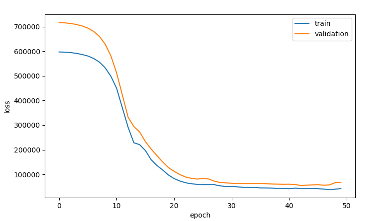
plt.plot(history.history['loss'])
plt.plot(history.history['val_loss'])
plt.xlabel('epoch')
plt.ylabel('loss')
plt.legend(['train', 'validation'], loc='best')
plt.show()
|
cs |
위 소스코드를 실행시키면 아래와 같은 출력값을 얻을 수 있다.
반응형
'머신러닝_딥러닝 > Tensorflow + Keras' 카테고리의 다른 글
| (Tensorflow 2.x) LSTM & GRU (0) | 2021.11.14 |
|---|---|
| (Tensorflow 2.x) RNN (0) | 2021.11.14 |
| (Tensorflow 2.x) 함수형 API (0) | 2021.10.23 |
| (Tensorflow 2.x) CNN 3탄 (Transfer Learning) (0) | 2021.10.23 |
| (Tensorflow 2.x) CNN 2탄 (With Garbage Classification) (0) | 2021.10.23 |